Raw Input Data
The data you'll be working with has been preprocessed from CSVs that looks like this:
| timestamp | displacement | yaw_rate | acceleration |
|---|---|---|---|
| 0.0 | 0 | 0.0 | 0.0 |
| 0.25 | 0.0 | 0.0 | 19.6 |
| 0.5 | 1.225 | 0.0 | 19.6 |
| 0.75 | 3.675 | 0.0 | 19.6 |
| 1.0 | 7.35 | 0.0 | 19.6 |
| 1.25 | 12.25 | 0.0 | 0.0 |
| 1.5 | 17.15 | -2.82901631903 | 0.0 |
| 1.75 | 22.05 | -2.82901631903 | 0.0 |
| 2.0 | 26.95 | -2.82901631903 | 0.0 |
| 2.25 | 31.85 | -2.82901631903 | 0.0 |
| 2.5 | 36.75 | -2.82901631903 | 0.0 |
| 2.75 | 41.65 | -2.82901631903 | 0.0 |
| 3.0 | 46.55 | -2.82901631903 | 0.0 |
| 3.25 | 51.45 | -2.82901631903 | 0.0 |
| 3.5 | 56.35 | -2.82901631903 | 0.0 |
This data is currently saved in a file called trajectory_example.pickle. It can be loaded using a helper function we've provided (demonstrated below):
from helpers import process_data

data_list = process_data("trajectory_example.pickle")

for entry in data_list:
    print(entry)
as you can see, each entry in data_list contains four fields. Those fields correspond to timestamp (seconds), displacement (meters), yaw_rate (rads / sec), and acceleration (m/s/s).
The Point of this Project!
Data tells a story but you have to know how to find it!
Contained in the data above is all the information you need to reconstruct a fairly complex vehicle trajectory. After processing this exact data, it's possible to generate this plot of the vehicle's X and Y position:
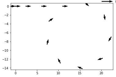
as you can see, this vehicle first accelerates forwards and then turns right until it almost completes a full circle turn.
Data Explained
timestamp - Timestamps are all measured in seconds. The time between successive timestamps ($\Delta t$) will always be the same within a trajectory's data set (but not between data sets).
displacement - Displacement data from the odometer is in meters and gives the total distance traveled up to this point.
yaw_rate - Yaw rate is measured in radians per second with the convention that positive yaw corresponds to counter-clockwise rotation.
acceleration - Acceleration is measured in $\frac{m/s}{s}$ and is always in the direction of motion of the vehicle (forward).
NOTE - you may not need to use all of this data when reconstructing vehicle trajectories.
Your Job
Your job is to complete the following functions, all of which take a processed data_list (with $N$ entries, each $\Delta t$ apart) as input:
get_speeds- returns a length $N$ list where entry $i$ contains the speed ($m/s$) of the vehicle at $t = i \times \Delta t$get_headings- returns a length $N$ list where entry $i$ contains the heading (radians, $0 \leq \theta < 2\pi$) of the vehicle at $t = i \times \Delta t$get_x_y- returns a length $N$ list where entry $i$ contains an(x, y)tuple corresponding to the $x$ and $y$ coordinates (meters) of the vehicle at $t = i \times \Delta t$show_x_y- generates an x vs. y scatter plot of vehicle positions.
# I've provided a solution file called solution.py
# You are STRONGLY encouraged to NOT look at the code
# until after you have solved this yourself.
#
# You SHOULD, however, feel free to USE the solution
# functions to help you understand what your code should
# be doing. For example...
from helpers import process_data
import solution

data_list = process_data("trajectory_example.pickle")
solution.show_x_y(data_list)

# What about the other trajectories?

three_quarter_turn_data = process_data("trajectory_1.pickle")
solution.show_x_y(three_quarter_turn_data, increment=10)

merge_data = process_data('trajectory_2.pickle')
solution.show_x_y(merge_data,increment=10)

parallel_park = process_data("trajectory_3.pickle")
solution.show_x_y(parallel_park,increment=5)

How do you make those cool arrows?!
I did a Google search for "python plot grid of arrows" and the second result led me to some demonstration code that was really helpful.
Testing Correctness
Testing code is provided at the bottom of this notebook. Note that only get_speeds, get_x_y, and get_headings are tested automatically. You will have to "test" your show_x_y function by manually comparing your plots to the expected plots.
Initial Vehicle State
The vehicle always begins with all state variables equal to zero. This means x, y, theta (heading), speed, yaw_rate, and acceleration are 0 at t=0.
Your Code!
Complete the functions in the cell below. I recommend completing them in the order shown. Use the cells at the end of the notebook to test as you go.
from math import cos, sin, pi
import matplotlib.pyplot as plt
import warnings
warnings.filterwarnings('ignore')

# Define column indicies in data array data_list
timestamp_index = 0
displacement_index = 1
yaw_rate_index = 2
acceleration_index = 3

def get_speeds(data_list):
    """
    Converts the data_list to a list of speeds at a given time stamps by keeping
    track of the current speed and adjusting it by the acceleration and time delta

    Return:  The list of speeds
    """
    speed = 0.0

    speeds = [speed]
    for index in range(1,len(data_list)):
        last_row = data_list[index-1]
        row = data_list[index]

        time = row[timestamp_index]-last_row[timestamp_index]
        acceleration = row[acceleration_index]
        speed += time*acceleration
        speeds.append(speed)

    return speeds

def get_headings(data_list):
    """
    Converts the data_list to a list of headings by keeping track of the current
    heading and adjusting it by the yaw_rate multiplied by time_delta.

    Return: The current heading at each time stamp in degree
    """
    heading = 0.0
    headings = [heading]

    for index in range(1,len(data_list)):
        last_row = data_list[index-1]
        row = data_list[index]

        time = row[timestamp_index]-last_row[timestamp_index]
        diff = row[yaw_rate_index]
        heading += time*diff
        headings.append(heading)

    return headings

def get_x_y(data_list):
    """
    Converts the data_list to a list of coordinates by keeping track of the
    current position and adjusting it using the known heading, displacement
    and time delta.

    Return: The list of vehicle coordinates
    """

    headings = get_headings(data_list)

    x = 0
    y = 0

    positions = [(x,y)]

    for index in range(1,len(data_list)):

        positions.append((x,y))

        last_row = data_list[index-1]
        row = data_list[index]

        time = row[timestamp_index]-last_row[timestamp_index]
        move_diff = row[displacement_index]-last_row[displacement_index]
        heading = headings[index]

        x += cos(heading)*move_diff
        y += sin(heading)*move_diff

    return positions

def show_x_y(data_list):
    """
    Shows the vehicle's position and movement direction at all time stamps
    """

    positions = get_x_y(data_list)
    headings = get_headings(data_list)

    X = [row[0] for row in positions]
    Y = [row[1] for row in positions]
    U = [cos(heading) for heading in headings]
    V = [sin(heading) for heading in headings]

    plt.figure()
    plt.title('Trajectory visualization')
    plt.axes().set_aspect('equal')
    Q = plt.quiver(X, Y, U, V, units='width')
    qk = plt.quiverkey(Q, 0.9, 0.9, 2, r'$2 \frac{m}{s}$', labelpos='E', coordinates='figure')
    plt.show()

    return
Testing
Test your functions by running the cells below.
from testing import test_get_speeds, test_get_x_y, test_get_headings

test_get_speeds(get_speeds)
test_get_x_y(get_x_y)
test_get_headings(get_headings)
show_x_y(data_list)
