Creating a Filter, Edge Detection
Import resources and display image
In [1]:
import matplotlib.pyplot as plt
import matplotlib.image as mpimg

import cv2
import numpy as np

%matplotlib inline

# Read in the image
image = mpimg.imread('images/curved_lane.jpg')

plt.imshow(image)
Out[1]:

Convert the image to grayscale
In [2]:
# Convert to grayscale for filtering
gray = cv2.cvtColor(image, cv2.COLOR_RGB2GRAY)

plt.imshow(gray, cmap='gray')
Out[2]:

TODO: Create a custom kernel
Below, you've been given one common type of edge detection filter: a Sobel operator.
The Sobel filter is very commonly used in edge detection and in finding patterns in intensity in an image. Applying a Sobel filter to an image is a way of taking (an approximation) of the derivative of the image in the x or y direction, separately. The operators look as follows.
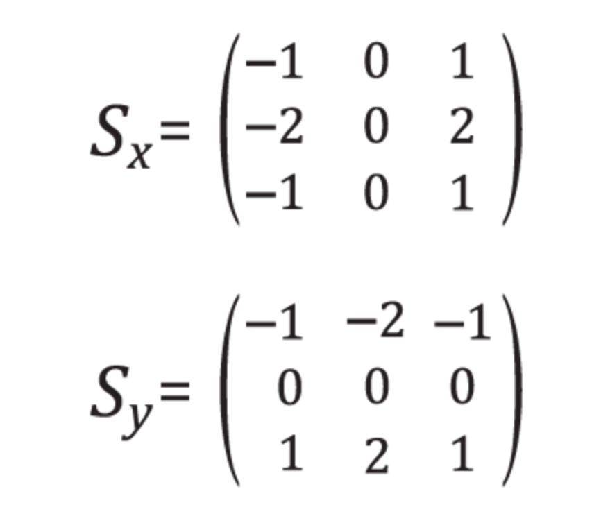
It's up to you to create a Sobel x operator and apply it to the given image.
For a challenge, see if you can put the image through a series of filters: first one that blurs the image (takes an average of pixels), and then one that detects the edges.
In [36]:
# Create a custom kernel

# 3x3 array for edge detection
sobel_y = np.array([[ -1, -2, -1],
                   [ 0, 0, 0],
                   [ 1, 2, 1]])

## TODO: Create and apply a Sobel x operator
sobel_x = np.array([[ -1, 0, 1],
                   [ -2, 0, 2],
                   [ -1, 0, 1]])

# Filter the image using filter2D, which has inputs: (grayscale image, bit-depth, kernel)
filtered_image = cv2.filter2D(gray, -1, sobel_y)

# Filter the image using filter2D, which has inputs: (grayscale image, bit-depth, kernel)
filtered_image_2 = cv2.filter2D(gray, -1, sobel_x)

plt.figure(figsize = (15,15))
plt.imshow(filtered_image, cmap='gray')
plt.title("sobel y")
plt.show()

plt.figure(figsize = (15,15))
plt.imshow(filtered_image_2, cmap='gray')
plt.title("sobel x")
plt.show()

blur_filter = np.array([[ 0.05, 0.2, 0.05],
                        [ 0.2, 0.2, 0.2],
                        [ 0.05, 0.2, 0.05]])

# Filter the image using filter2D, which has inputs: (grayscale image, bit-depth, kernel)
filtered_image_blur = cv2.filter2D(gray, -1, blur_filter)

plt.figure(figsize = (15,15))
plt.imshow(filtered_image_blur, cmap='gray')
plt.title("blur")
plt.show()

edge_detection = np.array([[ 0.0, -1, 0],
                        [ -1, 4, -1],
                        [ 0, -1, 0]])

# Filter the image using filter2D, which has inputs: (grayscale image, bit-depth, kernel)
filtered_image_edges = cv2.filter2D(filtered_image_blur, -1, edge_detection)

plt.figure(figsize = (15,15))
plt.imshow(filtered_image_edges, cmap='gray')
plt.title("edge detection")
plt.show()


Test out other filters!
You're encouraged to create other kinds of filters and apply them to see what happens! As an optional exercise, try the following:
- Create a filter with decimal value weights.
- Create a 5x5 filter
- Apply your filters to the other images in the
imagesdirectory.
In [34]:
# Read in the image
image_2 = mpimg.imread('images/white_lines.jpg')

# Convert to grayscale for filtering
gray_2 = cv2.cvtColor(image_2, cv2.COLOR_RGB2GRAY)

plt.imshow(gray_2, cmap='gray')
plt.show()

edge_detection_2 = [[0,0,-2.5,0,0],
                    [0,0,-1,0,0],
                    [-2.5,-1,12,-1,-2.5],
                    [0,0,-1,0,0],
                    [0,0,-2.5,0,0]]
edge_detection_2 = np.array(edge_detection_2)

# Filter the image using filter2D, which has inputs: (grayscale image, bit-depth, kernel)
filtered_image_edges_2 = cv2.filter2D(gray_2, -1, edge_detection_2)

plt.figure(figsize = (15,15))
plt.imshow(filtered_image_edges_2, cmap='gray')
plt.show()

