Traffic Light Classifier
In this project, you’ll use your knowledge of computer vision techniques to build a classifier for images of traffic lights! You'll be given a dataset of traffic light images in which one of three lights is illuminated: red, yellow, or green.
In this notebook, you'll pre-process these images, extract features that will help us distinguish the different types of images, and use those features to classify the traffic light images into three classes: red, yellow, or green. The tasks will be broken down into a few sections:
Loading and visualizing the data. The first step in any classification task is to be familiar with your data; you'll need to load in the images of traffic lights and visualize them!
Pre-processing. The input images and output labels need to be standardized. This way, you can analyze all the input images using the same classification pipeline, and you know what output to expect when you eventually classify a new image.
Feature extraction. Next, you'll extract some features from each image that will help distinguish and eventually classify these images.
Classification and visualizing error. Finally, you'll write one function that uses your features to classify any traffic light image. This function will take in an image and output a label. You'll also be given code to determine the accuracy of your classification model.
Evaluate your model. To pass this project, your classifier must be >90% accurate and never classify any red lights as green; it's likely that you'll need to improve the accuracy of your classifier by changing existing features or adding new features. I'd also encourage you to try to get as close to 100% accuracy as possible!
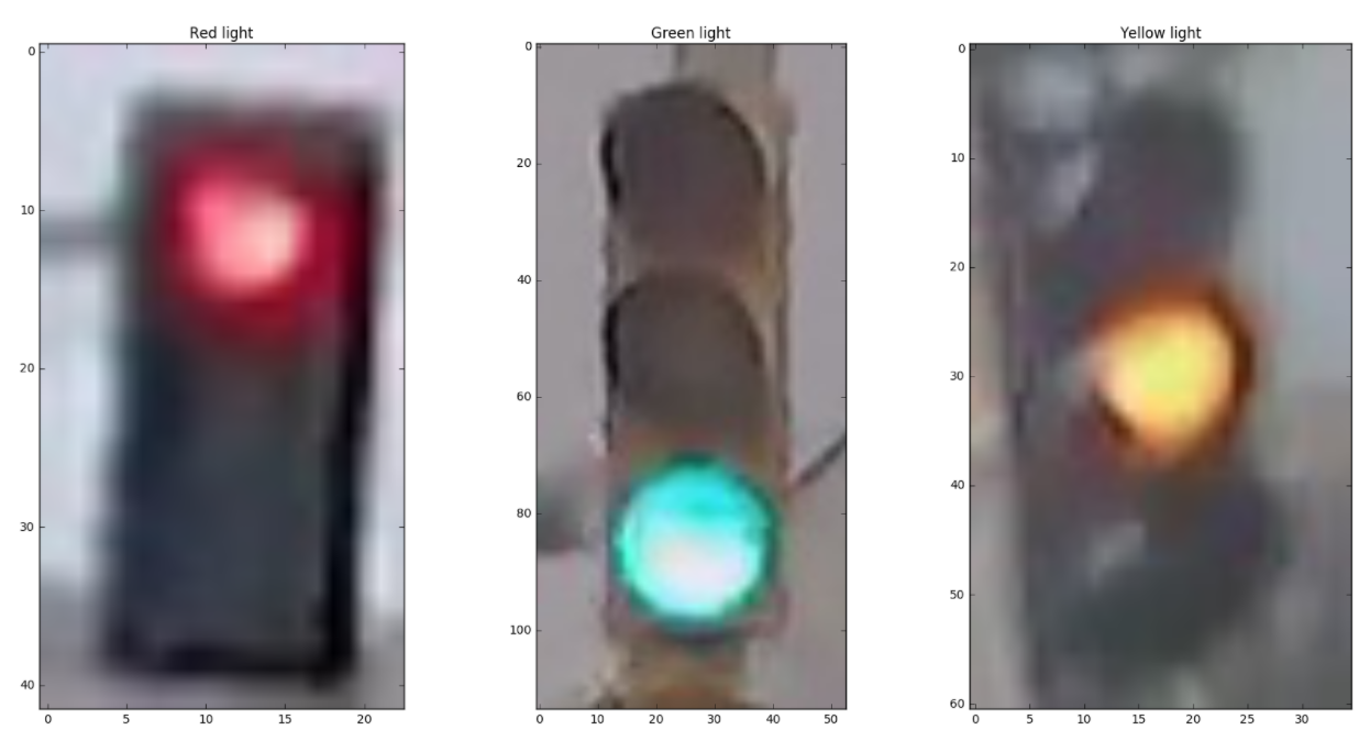
Here are some sample images from the dataset (from left to right: red, green, and yellow traffic lights):
Here's what you need to know to complete the project:
Some template code has already been provided for you, but you'll need to implement additional code steps to successfully complete this project. Any code that is required to pass this project is marked with '(IMPLEMENTATION)' in the header. There are also a couple of questions about your thoughts as you work through this project, which are marked with '(QUESTION)' in the header. Make sure to answer all questions and to check your work against the project rubric to make sure you complete the necessary classification steps!
Your project submission will be evaluated based on the code implementations you provide, and on two main classification criteria. Your complete traffic light classifier should have:
- Greater than 90% accuracy
- Never classify red lights as green
1. Loading and Visualizing the Traffic Light Dataset
This traffic light dataset consists of 1484 number of color images in 3 categories - red, yellow, and green. As with most human-sourced data, the data is not evenly distributed among the types. There are:
- 904 red traffic light images
- 536 green traffic light images
- 44 yellow traffic light images
Note: All images come from this MIT self-driving car course and are licensed under a Creative Commons Attribution-ShareAlike 4.0 International License.
Import resources
Before you get started on the project code, import the libraries and resources that you'll need.
import cv2 # computer vision library
import helpers # helper functions

import random
import numpy as np
import matplotlib.pyplot as plt
import matplotlib.image as mpimg # for loading in images

%matplotlib inline
Training and Testing Data
All 1484 of the traffic light images are separated into training and testing datasets.
- 80% of these images are training images, for you to use as you create a classifier.
- 20% are test images, which will be used to test the accuracy of your classifier.
- All images are pictures of 3-light traffic lights with one light illuminated.
Define the image directories
First, we set some variables to keep track of some where our images are stored:
IMAGE_DIR_TRAINING: the directory where our training image data is stored
IMAGE_DIR_TEST: the directory where our test image data is stored# Image data directories
IMAGE_DIR_TRAINING = "traffic_light_images/training/"
IMAGE_DIR_TEST = "traffic_light_images/test/"
Load the datasets
These first few lines of code will load the training traffic light images and store all of them in a variable, IMAGE_LIST. This list contains the images and their associated label ("red", "yellow", "green").
You are encouraged to take a look at the load_dataset function in the helpers.py file. This will give you a good idea about how lots of image files can be read in from a directory using the glob library. The load_dataset function takes in the name of an image directory and returns a list of images and their associated labels.
For example, the first image-label pair in IMAGE_LIST can be accessed by index:
IMAGE_LIST[0][:].
# Using the load_dataset function in helpers.py
# Load training data
IMAGE_LIST = helpers.load_dataset(IMAGE_DIR_TRAINING)
Visualize the Data
The first steps in analyzing any dataset are to 1. load the data and 2. look at the data. Seeing what it looks like will give you an idea of what to look for in the images, what kind of noise or inconsistencies you have to deal with, and so on. This will help you understand the image dataset, and understanding a dataset is part of making predictions about the data.
Visualize the input images
Visualize and explore the image data! Write code to display an image in IMAGE_LIST:
- Display the image
- Print out the shape of the image
- Print out its corresponding label
See if you can display at least one of each type of traffic light image – red, green, and yellow — and look at their similarities and differences.
## TODO: Write code to display an image in IMAGE_LIST (try finding a yellow traffic light!)
## TODO: Print out 1. The shape of the image and 2. The image's label

# ------------------- Global Definitions -------------------

# Definition of the 3 possible traffic light states and theirs label
tl_states = ['red', 'yellow', 'green']
tl_state_red = 0
tl_state_yellow = 1
tl_state_green = 2
tl_state_count = 3
tl_state_red_string = tl_states[tl_state_red]
tl_state_yellow_string = tl_states[tl_state_yellow]
tl_state_green_string = tl_states[tl_state_green]

# Index of image and label in image set
image_data_image_index = 0
image_data_label_index = 1

# Normalized image size
default_image_size = 32

# ---------------- End of Global Definitions ---------------

fig = plt.figure(figsize=(20,40))

example_count = 24
if example_count>len(IMAGE_LIST):
    example_count = len(IMAGE_LIST)

chosen = set()

# print 24 random examples, prevent double choice
for example_index in range(example_count):
    tries = 0

    while tries<2:
        index = 0
        tries += 1
        if example_index==0: # first choice should be a yellow light
            for iterator in range(len(IMAGE_LIST)):
                if IMAGE_LIST[iterator][image_data_label_index]==tl_state_yellow_string:
                    index = iterator
                    break
        else: # all other choices are random
            index = random.randint(0, len(IMAGE_LIST)-1)

        if index in chosen: # try a second time if chosen already
            continue
        chosen.add(index)

    example_image = IMAGE_LIST[index][image_data_image_index]
    result = "{}, shape: {}".format(IMAGE_LIST[index][image_data_label_index],example_image.shape)
    ax = fig.add_subplot(example_count, 4, example_index+1, title=result)
    ax.imshow(example_image.squeeze())

fig.tight_layout(pad=0.7)

2. Pre-process the Data
After loading in each image, you have to standardize the input and output!
Input
This means that every input image should be in the same format, of the same size, and so on. We'll be creating features by performing the same analysis on every picture, and for a classification task like this, it's important that similar images create similar features!
Output
We also need the output to be a label that is easy to read and easy to compare with other labels. It is good practice to convert categorical data like "red" and "green" to numerical data.
A very common classification output is a 1D list that is the length of the number of classes - three in the case of red, yellow, and green lights - with the values 0 or 1 indicating which class a certain image is. For example, since we have three classes (red, yellow, and green), we can make a list with the order: [red value, yellow value, green value]. In general, order does not matter, we choose the order [red value, yellow value, green value] in this case to reflect the position of each light in descending vertical order.
A red light should have the label: [1, 0, 0]. Yellow should be: [0, 1, 0]. Green should be: [0, 0, 1]. These labels are called one-hot encoded labels.
(Note: one-hot encoding will be especially important when you work with machine learning algorithms).
(IMPLEMENTATION): Standardize the input images
- Resize each image to the desired input size: 32x32px.
- (Optional) You may choose to crop, shift, or rotate the images in this step as well.
It's very common to have square input sizes that can be rotated (and remain the same size), and analyzed in smaller, square patches. It's also important to make all your images the same size so that they can be sent through the same pipeline of classification steps!
# This function should take in an RGB image and return a new, standardized version
def standardize_input(image):

    ## TODO: Resize image and pre-process so that all "standard" images are the same size
    standard_im = cv2.resize(image.astype('uint8'), dsize=(default_image_size, default_image_size))

    return standard_im
Standardize the output
With each loaded image, we also specify the expected output. For this, we use one-hot encoding.
- One-hot encode the labels. To do this, create an array of zeros representing each class of traffic light (red, yellow, green), and set the index of the expected class number to 1.
Since we have three classes (red, yellow, and green), we have imposed an order of: [red value, yellow value, green value]. To one-hot encode, say, a yellow light, we would first initialize an array to [0, 0, 0] and change the middle value (the yellow value) to 1: [0, 1, 0].
## TODO: One hot encode an image label
## Given a label - "red", "green", or "yellow" - return a one-hot encoded label

# Examples:
# one_hot_encode("red") should return: [1, 0, 0]
# one_hot_encode("yellow") should return: [0, 1, 0]
# one_hot_encode("green") should return: [0, 0, 1]

def one_hot_encode(label):

    ## TODO: Create a one-hot encoded label that works for all classes of traffic lights
    one_hot_encoded = [0, 0, 0]
    for state_index in range(tl_state_count):
        if label==tl_states[state_index]:
            one_hot_encoded[state_index] = 1

    return one_hot_encoded

print(one_hot_encode("red"))
print(one_hot_encode("yellow"))
print(one_hot_encode("green"))
Testing as you Code
After programming a function like this, it's a good idea to test it, and see if it produces the expected output. In general, it's good practice to test code in small, functional pieces, after you write it. This way, you can make sure that your code is correct as you continue to build a classifier, and you can identify any errors early on so that they don't compound.
All test code can be found in the file test_functions.py. You are encouraged to look through that code and add your own testing code if you find it useful!
One test function you'll find is: test_one_hot(self, one_hot_function) which takes in one argument, a one_hot_encode function, and tests its functionality. If your one_hot_label code does not work as expected, this test will print ot an error message that will tell you a bit about why your code failed. Once your code works, this should print out TEST PASSED.
# Importing the tests
import test_functions
tests = test_functions.Tests()

# Test for one_hot_encode function
tests.test_one_hot(one_hot_encode)
Construct a STANDARDIZED_LIST of input images and output labels.
This function takes in a list of image-label pairs and outputs a standardized list of resized images and one-hot encoded labels.
This uses the functions you defined above to standardize the input and output, so those functions must be complete for this standardization to work!
def standardize(image_list):

    # Empty image data array
    standard_list = []

    # Iterate through all the image-label pairs
    for item in image_list:
        image = item[0]
        label = item[1]

        # Standardize the image
        standardized_im = standardize_input(image)

        # One-hot encode the label
        one_hot_label = one_hot_encode(label)

        # Append the image, and it's one hot encoded label to the full, processed list of image data
        standard_list.append((standardized_im, one_hot_label))

    return standard_list

# Standardize all training images
STANDARDIZED_LIST = standardize(IMAGE_LIST)
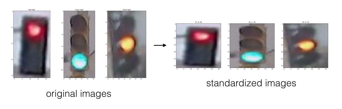
Visualize the standardized data
Display a standardized image from STANDARDIZED_LIST and compare it with a non-standardized image from IMAGE_LIST. Note that their sizes and appearance are different!
# TODO: Display a standardized image and its label

fig = plt.figure(figsize=(20,40))

# 12 example pairs
example_count = 12
if example_count>len(IMAGE_LIST):
    example_count = len(IMAGE_LIST)
total_count = example_count*2

chosen = set() # use set to prevent double random selection

for example_index in range(example_count):

    tries = 0
    index = 0

    # select next image
    while tries<2:
        tries += 1
        index = random.randint(0, len(IMAGE_LIST)-1)

        if index in chosen:
            continue
        chosen.add(index)

    eff_index = example_index*2

    # print original
    example_image = IMAGE_LIST[index][image_data_image_index]
    result = "{} {}".format(IMAGE_LIST[index][image_data_label_index],example_image.shape)
    ax = fig.add_subplot(total_count, 4, eff_index+1, title=result)
    ax.imshow(example_image.squeeze())

    # print standardized counterpiece
    eff_index += 1
    example_image = STANDARDIZED_LIST[index][image_data_image_index]
    result = "{} {}".format(STANDARDIZED_LIST[index][image_data_label_index],example_image.shape)
    ax = fig.add_subplot(total_count, 4, eff_index+1, title=result)
    ax.imshow(example_image.squeeze())

fig.tight_layout(pad=0.7)

3. Feature Extraction
You'll be using what you now about color spaces, shape analysis, and feature construction to create features that help distinguish and classify the three types of traffic light images.
You'll be tasked with creating one feature at a minimum (with the option to create more). The required feature is a brightness feature using HSV color space:
A brightness feature.
- Using HSV color space, create a feature that helps you identify the 3 different classes of traffic light.
- You'll be asked some questions about what methods you tried to locate this traffic light, so, as you progress through this notebook, always be thinking about your approach: what works and what doesn't?
(Optional): Create more features!
Any more features that you create are up to you and should improve the accuracy of your traffic light classification algorithm! One thing to note is that, to pass this project you must never classify a red light as a green light because this creates a serious safety risk for a self-driving car. To avoid this misclassification, you might consider adding another feature that specifically distinguishes between red and green lights.
These features will be combined near the end of his notebook to form a complete classification algorithm.
Creating a brightness feature
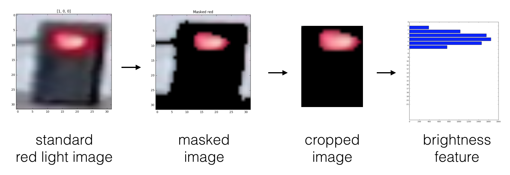
There are a number of ways to create a brightness feature that will help you characterize images of traffic lights, and it will be up to you to decide on the best procedure to complete this step. You should visualize and test your code as you go.
Pictured below is a sample pipeline for creating a brightness feature (from left to right: standardized image, HSV color-masked image, cropped image, brightness feature):
RGB to HSV conversion
Below, a test image is converted from RGB to HSV colorspace and each component is displayed in an image.
# Convert and image to HSV colorspace
# Visualize the individual color channels

image_num = 0
test_im = STANDARDIZED_LIST[image_num][0]
test_label = STANDARDIZED_LIST[image_num][1]

# Convert to HSV
hsv = cv2.cvtColor(test_im, cv2.COLOR_RGB2HSV)

# Print image label
print('Label [red, yellow, green]: ' + str(test_label))

# HSV channels
h = hsv[:,:,0]
s = hsv[:,:,1]
v = hsv[:,:,2]

# Plot the original image and the three channels
f, (ax1, ax2, ax3, ax4) = plt.subplots(1, 4, figsize=(20,10))
ax1.set_title('Standardized image')
ax1.imshow(test_im)
ax2.set_title('H channel')
ax2.imshow(h, cmap='gray')
ax3.set_title('S channel')
ax3.imshow(s, cmap='gray')
ax4.set_title('V channel')
ax4.imshow(v, cmap='gray')

(IMPLEMENTATION): Create a brightness feature that uses HSV color space
Write a function that takes in an RGB image and returns a 1D feature vector and/or single value that will help classify an image of a traffic light. The only requirement is that this function should apply an HSV colorspace transformation, the rest is up to you.
From this feature, you should be able to estimate an image's label and classify it as either a red, green, or yellow traffic light. You may also define helper functions if they simplify your code.
import math

# crop settings, remove as much as possible to prevent too much influence by objects near the traffic light
crop_left_right = 12
crop_top_bottom = 3

def mask_image_get_brightness_vector(rgb_image):
    """
    Tries to identify highlights within the traffic light's inner region and removes a vector with the
    brightness history from top to bottom

    rgb_image: An RGB image of a traffic light
    return: The history vector
    """
    hsv = cv2.cvtColor(rgb_image, cv2.COLOR_RGB2HSV)
    hsv = hsv[crop_top_bottom:default_image_size-crop_top_bottom,crop_left_right:default_image_size-crop_left_right]
    brightness = hsv[:,:,2]
    summed_brightness = np.sum(brightness, axis=1)

    return (brightness,hsv[:,:,1],summed_brightness)

## TODO: Create a brightness feature that takes in an RGB image and outputs a feature vector and/or value
## This feature should use HSV colorspace values
def create_feature(rgb_image):
    """
    Creates a brightness feature using the image of a traffic light


    rgb_image: An RGB image of a traffic light
    return: (The brightness mask, The saturation mask, The brightness history vector from top to bottom)"""
    (img_bright, img_sat, sb) = mask_image_get_brightness_vector(rgb_image)

    ## TODO: Create and return a feature value and/or vector
    feature = sb

    return feature

# Show an example image

image_num = random.randint(0,len(STANDARDIZED_LIST)-1)
print("Image index: {}".format(image_num))
test_im = STANDARDIZED_LIST[image_num][0]
test_label = STANDARDIZED_LIST[image_num][1]
print(test_label)

img_bright, img_sat, sb = mask_image_get_brightness_vector(test_im)

cropped_org = test_im[crop_top_bottom:default_image_size-crop_top_bottom,crop_left_right:default_image_size-crop_left_right]

# Show details of example image
f, (org, bright, sat, b) = plt.subplots(1, 4, figsize=(10,5))
org.set_title("Original")
bright.set_title("Brightness")
sat.set_title("Saturation")
b.set_title("Brightness vector")
org.imshow(cropped_org)
bright.imshow(img_bright, cmap='gray')
sat.imshow(img_sat, cmap='gray')
b.barh(range(len(sb)), sb)
b.invert_yaxis()
plt.show()

(Optional) Create more features to help accurately label the traffic light images
# (Optional) Add more image analysis and create more features

def get_color_dominance(rgb_image):
    """This function searches for a very dominant red, yellow or green color within the traffic lights
    inner image region and independent of it's position

    rgb_image: The traffic light image
    return: A vector containing the percentage of red, yellow and green, (NOT RGB channels!) within the image
    """

    agg_colors = [0,0,0]

    cropped_image = rgb_image[crop_top_bottom:default_image_size-crop_top_bottom,crop_left_right:default_image_size-crop_left_right]

    threshold_min = 140
    threshold_min_b = 120
    threshold_rel = 0.75
    total_pixels = len(cropped_image)*len(cropped_image[1])

    for row_index in range(len(cropped_image)):
        cur_row = cropped_image[row_index]
        for col_index in range(len(cropped_image[0])):
            pixel = cur_row[col_index]
            if pixel[0]>threshold_min and pixel[1]<pixel[0]*threshold_rel and pixel[2]<pixel[0]*threshold_rel:
                agg_colors[0] += 1
            if pixel[0]>threshold_min and pixel[1]>threshold_min and pixel[2]<pixel[0]*threshold_rel:
                agg_colors[1] += 1
            if pixel[1]>threshold_min and pixel[0]<pixel[1]*threshold_rel and pixel[2]>threshold_min_b:
                agg_colors[2] += 1

    agg_colors = np.array(agg_colors)/float(total_pixels)

    return agg_colors

# Display an example image
image_num = random.randint(0,len(STANDARDIZED_LIST)-1)
print("Image index: {}".format(image_num))
test_im = STANDARDIZED_LIST[image_num][0]
test_label = STANDARDIZED_LIST[image_num][1]
print(test_label)

img_bright, img_sat, sb = mask_image_get_brightness_vector(test_im)

cropped_org = test_im[crop_top_bottom:default_image_size-crop_top_bottom,crop_left_right:default_image_size-crop_left_right]

agg_colors = get_color_dominance(test_im)

# Try to identify the image by dominant colors
dominant = np.argmax(agg_colors)

# Thresholds for dominant colors
dominant_sure_threshold = 0.15
dominant_threshold = 0.015

if agg_colors[dominant]>dominant_threshold:
    print("By dominance detected color: {} ({})".format(tl_states[dominant],agg_colors))
else:
    print("No dominant color detected")

# Show details of example image
f, (org, bright, sat, b) = plt.subplots(1, 4, figsize=(10,5))
org.set_title("Original")
bright.set_title("Brightness")
sat.set_title("Saturation")
b.set_title("Brightness vector")
org.imshow(cropped_org)
bright.imshow(img_bright, cmap='gray')
sat.imshow(img_sat, cmap='gray')
b.barh(range(len(sb)), sb)
b.invert_yaxis()
plt.show()

(QUESTION 1): How do the features you made help you distinguish between the 3 classes of traffic light images?
Answer:
I basically tried to realize the same technique most human drivers would use.
First I searched for a dominating color, majorly red was very very flashy, even in very bright images, so deciding that a traffic light is red if about 20% of the cropped traffic light image is red was a very safe bet.
Much more difficult it was with the color green which seems to be very very hard detectable just by color and in difference to "Super Mario Green" also has a large portion of blue making it even more difficult to distinguish it from white or bright objects close to the the traffic light.
As already proposed and demanded I also used the brightness map, converted it into a vector and then divided the vector into three sections for red, yellow and green. Basically that's the way every red/green blind human had to decide as well.
As already mentioned a "sure red" though still was more important in the final decision, the brightness map though helped a lot to decide between red and orange and to find green traffic lights in general.
4. Classification and Visualizing Error
Using all of your features, write a function that takes in an RGB image and, using your extracted features, outputs whether a light is red, green or yellow as a one-hot encoded label. This classification function should be able to classify any image of a traffic light!
You are encouraged to write any helper functions or visualization code that you may need, but for testing the accuracy, make sure that this estimate_label function returns a one-hot encoded label.
# This function should take in RGB image input
# Analyze that image using your feature creation code and output a one-hot encoded label
def estimate_label(rgb_image):

    ## TODO: Extract feature(s) from the RGB image and use those features to
    ## classify the image and output a one-hot encoded label

    # get the brightness vector feature first, this is a great fallback in any case
    feature = create_feature(rgb_image)

    # search for a visually dominant color as well
    dominant = get_color_dominance(rgb_image)

    max_dominant = np.argmax(dominant)

    one_hot = [0,0,0]

    maxc = len(feature)//3*3
    div = maxc//3
    prob = [np.sum(feature[0:div]), np.sum(feature[div:2*div]), np.sum(feature[2*div:3*div])]

    one_hot[np.argmax(prob)] = 1

    red_yellow_tolerance = 0.8

    # if one color is so dominant that it's not disusable: take it
    # if the algorithm is unsure combine it with the knowledge obtained by the brightness vector
    if(dominant[max_dominant]>dominant_threshold):  # is there a very dominant color ?
        if max_dominant==tl_state_red or max_dominant==tl_state_yellow:
            val = dominant[max_dominant]
            scaled_val = val*red_yellow_tolerance
            if scaled_val<dominant[0] and scaled_val<dominant[1]:
                return one_hot

        one_hot = [0,0,0]
        one_hot[max_dominant] = 1
        return one_hot

    return one_hot

image_num = random.randint(0,len(STANDARDIZED_LIST)-1)
print("Image index: {}".format(image_num))
test_im = STANDARDIZED_LIST[image_num][0]

label = estimate_label(test_im)
print(label)
plt.imshow(test_im)

Testing the classifier
Here is where we test your classification algorithm using our test set of data that we set aside at the beginning of the notebook! This project will be complete once you've pogrammed a "good" classifier.
A "good" classifier in this case should meet the following criteria (and once it does, feel free to submit your project):
- Get above 90% classification accuracy.
- Never classify a red light as a green light.
Test dataset
Below, we load in the test dataset, standardize it using the standardize function you defined above, and then shuffle it; this ensures that order will not play a role in testing accuracy.
# Using the load_dataset function in helpers.py
# Load test data
TEST_IMAGE_LIST = helpers.load_dataset(IMAGE_DIR_TEST)

# Standardize the test data
STANDARDIZED_TEST_LIST = standardize(TEST_IMAGE_LIST)

# Shuffle the standardized test data
random.shuffle(STANDARDIZED_TEST_LIST)
Determine the Accuracy
Compare the output of your classification algorithm (a.k.a. your "model") with the true labels and determine the accuracy.
This code stores all the misclassified images, their predicted labels, and their true labels, in a list called MISCLASSIFIED. This code is used for testing and should not be changed.
# Constructs a list of misclassified images given a list of test images and their labels
# This will throw an AssertionError if labels are not standardized (one-hot encoded)

def get_misclassified_images(test_images):
    # Track misclassified images by placing them into a list
    misclassified_images_labels = []

    # Iterate through all the test images
    # Classify each image and compare to the true label
    for image in test_images:

        # Get true data
        im = image[0]
        true_label = image[1]
        assert(len(true_label) == 3), "The true_label is not the expected length (3)."

        # Get predicted label from your classifier
        predicted_label = estimate_label(im)
        assert(len(predicted_label) == 3), "The predicted_label is not the expected length (3)."

        # Compare true and predicted labels
        if(predicted_label != true_label):
            # If these labels are not equal, the image has been misclassified
            misclassified_images_labels.append((im, predicted_label, true_label))

    # Return the list of misclassified [image, predicted_label, true_label] values
    return misclassified_images_labels


# Find all misclassified images in a given test set
MISCLASSIFIED = get_misclassified_images(STANDARDIZED_TEST_LIST)

# Accuracy calculations
total = len(STANDARDIZED_TEST_LIST)
num_correct = total - len(MISCLASSIFIED)
accuracy = num_correct/total
opencv_accuracy = accuracy*100.0

print('Accuracy: ' + str(accuracy))
print("Number of misclassified images = " + str(len(MISCLASSIFIED)) +' out of '+ str(total))
Visualize the misclassified images
Visualize some of the images you classified wrong (in the MISCLASSIFIED list) and note any qualities that make them difficult to classify. This will help you identify any weaknesses in your classification algorithm.
# Visualize misclassified example(s)
## TODO: Display an image in the `MISCLASSIFIED` list
## TODO: Print out its predicted label - to see what the image *was* incorrectly classified as

fig = plt.figure(figsize=(20,40))

example_count = 24
if example_count>len(MISCLASSIFIED):
    example_count = len(MISCLASSIFIED)

chosen = set()

for cur_index in range(example_count):
    example_image = MISCLASSIFIED[cur_index][image_data_image_index]
    dom = get_color_dominance(example_image)
    result = "{} {} {}".format(MISCLASSIFIED[cur_index][1],MISCLASSIFIED[cur_index][2], dom)
    ax = fig.add_subplot(example_count, 4, cur_index+1, title=result)
    ax.imshow(example_image.squeeze())

fig.tight_layout(pad=0.7)

(Question 2): After visualizing these misclassifications, what weaknesses do you think your classification algorithm has? Please note at least two.
Answer:
It's major weakness is detecting green traffic lights on a very sunny day on which the camera either heavily overexposed the whole image including the traffic light or underexpoded it so it seemed (like in the two right images above) even for a human eye that it might be switched off.
In general green was the hardest of the three colors to detect, because it doesn't have a single really dominating and in other regions of the image rarely occuring component like the red. In consequence (as seen in the second image above) in an overexposed image the "foggy" red area of the traffic light will dominate the green ones, because in this case it's just an arrow which even less scores for the green region of the traffic light.
Another large weakness of my algorithm is out of question that it relies a lot on the matter that the images provided already contain the traffic light more or less in it's center. I think in practice when just receiving a video stream from an onboard camera the far harder part of detecting a traffic light's color would be to find the perfect bounding box for a traffic light at all.
Test if you classify any red lights as green
To pass this project, you must not classify any red lights as green! Classifying red lights as green would cause a car to drive through a red traffic light, so this red-as-green error is very dangerous in the real world.
The code below lets you test to see if you've misclassified any red lights as green in the test set. This test assumes that MISCLASSIFIED is a list of tuples with the order: [misclassified_image, predicted_label, true_label].
Note: this is not an all encompassing test, but its a good indicator that, if you pass, you are on the right track! This iterates through your list of misclassified examples and checks to see if any red traffic lights have been mistakenly labelled [0, 1, 0] (green).
# Importing the tests
import test_functions
tests = test_functions.Tests()

if(len(MISCLASSIFIED) > 0):
    # Test code for one_hot_encode function
    tests.test_red_as_green(MISCLASSIFIED)
else:
    print("MISCLASSIFIED may not have been populated with images.")
5. Improve your algorithm!
Submit your project after you have completed all implementations, answered all questions, AND when you've met the two criteria:
- Greater than 90% accuracy classification
- No red lights classified as green
If you did not meet these requirements (which is common on the first attempt!), revisit your algorithm and tweak it to improve light recognition -- this could mean changing the brightness feature, performing some background subtraction, or adding another feature!
Going Further (Optional Challenges)
If you found this challenge easy, I suggest you go above and beyond! Here are a couple optional (meaning you do not need to implement these to submit and pass the project) suggestions:
- (Optional) Aim for >95% classification accuracy. - Check :)
- (Optional) Some lights are in the shape of arrows; further classify the lights as round or arrow-shaped. - Soon :)
- (Optional) Add another feature and aim for as close to 100% accuracy as you can get! - Added the color dominance check, was 96% before, 98.65% is fine I guess, but will still try to catch at least two of the missed ones afterwards ;)
Optional part - Traffic light detection using deep learning
Because I am enrolled in the Deep Learning Foundations Nanodegree parallel to this one I was of course curious how much better or worser a totally automatically trained network would compete with my over many many hours finetuned version above.
After the "insane" accuracy rates of the other projects in the DLND it though did not really surprise me that it reached the 100% for this test set, the neural net easily adapted to the over and underexpoded image as shown below as well.
Part 1: Preparing Tensorflow compatible sets for training, validating and testing
# Prepare training set
y_train = []
x_train = []

for index in range(len(STANDARDIZED_LIST)):
    x_train.append(STANDARDIZED_LIST[index][0])
    y_train.append(STANDARDIZED_LIST[index][1])

x_train = np.array(x_train)
y_train = np.array(y_train)

# Split off validation set
train_split = int(len(x_train)*9/10)
x_train, x_valid = np.split(x_train, [train_split])
y_train, y_valid = np.split(y_train, [train_split])

# Load hidden testing set for real accuracy test
y_test = []
x_test = []

for index in range(len(STANDARDIZED_TEST_LIST)):
    x_test.append(STANDARDIZED_TEST_LIST[index][0])
    y_test.append(STANDARDIZED_TEST_LIST[index][1])

x_test = np.array(x_test)
y_test = np.array(y_test)
Model definition
For a fast training I have made very very good experiences with an 3-5 convolutional layers, each using a 3x3 kernel and increase filter count, in this case just layers because of the very small image size of 32. Each layer's data is batch normalized, the after the final conv layer the data is average pooled before densing it down to the count of categories, in our case the 3 traffic light modes.
from keras.layers import Conv2D, MaxPooling2D, GlobalAveragePooling2D
from keras.layers import Dropout, Flatten, Dense
from keras.models import Sequential
from keras.layers.normalization import BatchNormalization
from keras.callbacks import ModelCheckpoint

tlcat_model = Sequential()

tlcat_model.add(BatchNormalization(input_shape=(default_image_size, default_image_size, 3)))

tlcat_model.add(Conv2D(filters=16, kernel_size=3, activation='relu'))
tlcat_model.add(MaxPooling2D(pool_size=2))
tlcat_model.add(BatchNormalization())

tlcat_model.add(Conv2D(filters=32, kernel_size=3, activation='relu'))
tlcat_model.add(MaxPooling2D(pool_size=2))
tlcat_model.add(BatchNormalization())

tlcat_model.add(Conv2D(filters=64, kernel_size=3, activation='relu'))
tlcat_model.add(MaxPooling2D(pool_size=2))
tlcat_model.add(BatchNormalization())

tlcat_model.add(GlobalAveragePooling2D())

tlcat_model.add(Dense(3, activation='softmax')) # (red, yellow, green)
tlcat_model.summary()
tlcat_model.compile(optimizer='rmsprop', loss='categorical_crossentropy', metrics=['accuracy'])
Training the model
# train the model
checkpointer = ModelCheckpoint(filepath='model.weights.traffic_lights.hdf5', verbose=1,
                               save_best_only=True)
tlcat_model.fit(x_train, y_train, batch_size=64, epochs=20,
          validation_data=(x_valid, y_valid), callbacks=[checkpointer],
          verbose=2, shuffle=True)
tlcat_model.load_weights('model.weights.traffic_lights.hdf5')
# get index of predicted traffic light state for each image in test set
predictions = [np.argmax(tlcat_model.predict(np.expand_dims(feature, axis=0))) for feature in x_test]

# report test accuracy
test_accuracy = 100*np.sum(np.array(predictions)==np.argmax(y_test, axis=1))/len(predictions)
print('Test accuracy: %.4f%%' % test_accuracy)
Final test and presentation
fig = plt.figure(figsize=(10,40))

chosen = set()

print('OpenCV test accuracy   : %.4f%%' % opencv_accuracy)
print('Neural network accuracy: %.4f%%' % test_accuracy)

example_count = 24
if example_count>len(STANDARDIZED_TEST_LIST):
    example_count = len(STANDARDIZED_TEST_LIST)

for example_index in range(example_count):
    tries = 0
    index = 0

    while tries<2:
        tries += 1
        index = random.randint(0, len(STANDARDIZED_TEST_LIST)-1)

        if index in chosen:
            continue
        chosen.add(index)

    example_image = STANDARDIZED_TEST_LIST[index][image_data_image_index]

    light_state = np.argmax(tlcat_model.predict(np.expand_dims(example_image, axis=0)))

    result = tl_states[light_state]
    ax = fig.add_subplot(total_count, 4, example_index+1, title=result)
    ax.imshow(example_image.squeeze())

fig.tight_layout(pad=0.7)
